Special K Continued Fractions for Pi
Introduction
The purpose of this paper is to calculate the entropy of T. Schneider's continued fraction map, and to show the map has a natural extension which is Bernoulli. This is then used to study the behaviour of averages of convergents arising from Schneider's map. Schneider's map is usually defined on the p-adic field for the rational prime p, see [26]. In fact we work in a more general setting which we now describe. Let K denote a topological field. By this, we mean that the field K is a locally compact group under the addition, with respect to a topology. This ensures that there is a translation invariant Haar measure \(\mu \) on K, which is unique up to scalar multiplication. In the non-Archimedean examples that concern us in this paper, this topology will always be discrete. For an element \(a \in K\), we are now able to define its absolute value, as
$$\begin{aligned} |a| = \frac{\mu (aF)}{\mu (F)}, \end{aligned}$$
for every \(\mu \) measurable \(F \subseteq K\) of finite positive \(\mu \) measure. Let \({\mathbb {R}}_{\ge 0}\) denote the set of all non-negative real numbers. An absolute value is a function \(|.| : K \rightarrow {\mathbb {R}}_{\ge 0}\) such that (i) \(|a|= 0\) if and only if \(a=0\); (ii) \(|ab|= |a||b|\) for all \(a,b \in K\) and (iii) \( |a+b| \le |a| + |b|\) for all pairs \(a,b \in K\). The absolute value just defined gives rise to a metric defined by \(d(a,b) = |a-b|\) with \( a,b \in K\), whose topology coincides with original topology on the field K.
Topological fields come in two types. The first where (iii) can be replaced by the stronger condition (iii)* \(|a+b| \le \max (|a|, |b| ) \ a,b \in K\), called non-Archimedean fields and fields where (iii)* is not true called Archimedean spaces. In this paper, we shall concern ourselves solely with non-Archimedean fields. Another approach to defining a non-Archimedean field is via discrete valuations. Denote the real numbers by \({\mathbb {R}}\). Let \(K^*=K\backslash \{ 0 \}\). A map \(v : K ^*\rightarrow {\mathbb {R}}\) is a valuation if (a) \(v(K^*) \not = \{ 0 \}\); (b) \(v(xy) = v(x) + v(y)\) for \(x,y \in K\) and (c) \(v(x + y) \ge \min \{v(x), v(y) \}\). Two valuations v and cv, for \(c > 0\) a real constant, are called equivalent. We extend v to K formally by letting \(v(0) = \infty \). The image \( v(K^*)\) is an additive subgroup of \({\mathbb {R}}\) called the value group of v. If the value group is isomorphic to \({\mathbb {Z}}\), we say v is a discrete valuation. Here \({\mathbb {Z}}\) denotes the set of integers. If \(v(K^*) = {\mathbb {Z}}\), we call v a normalised discrete valuation. To our initial absolute value we associate the valuation described as follows. Pick \(0< \alpha < 1\) and write \(|a| = \alpha ^{v(a)}\), i.e., let \(v(a) = \log _{\alpha }| a|\). Then v(a) is a valuation, an additive version of |a|.
Let \( v : K^* \rightarrow {\mathbb {R}}\) be a valuation corresponding to the absolute value \( | . | : K \rightarrow {\mathbb {R}}_ {\ge 0}\). Then
$$\begin{aligned} {\mathcal {O}} ={\mathcal {O}}_v := \{ x \in K : v(x) \ge 0 \} = {\mathcal {O}} _K := \{ x \in K : |x| \le 1 \} \end{aligned}$$
is a ring, called the valuation ring of v and K is its field of fractions. The set of units in \({\mathcal {O}}\) is \({\mathcal {O}}^{\times } = \{ x \in K : v(x) = 0 \} = \{ x \in K : |x| = 1 \}\) and \({\mathcal {M}} = \{ x \in K : v(x) > 0 \} = \{ x \in K : |x| < 1 \}\) is an ideal in \({\mathcal {O}}\). Note \({\mathcal {O}} = {\mathcal {O}}^{\times } \cup {\mathcal {M}}\). Because \({\mathcal {M}}\) is a maximal ideal, we know \(k = { {\mathcal {O}}}/{\mathcal {M}}\) is a field, called the residue field of v or of K. In the sequel throughout this paper, we assume that k is a finite field. Suppose the valuation \(v : K^*\rightarrow {\mathbb {Z}}\) is normalised and discrete. Take \(\pi \in {\mathcal {M}}\) such that \(v(\pi ) = 1\). We call \(\pi \) a uniformizer. Then every \(x \in K\) can be written uniquely as \(x = u\pi ^n\) with \(u\in {\mathcal {O}}^{\times }\) and \(n\in {\mathbb {Z}}\). In particular every \(x \in {\mathcal {M}}\) can be written uniquely as \(x = u\pi ^n\) for a unit \(u \in {\mathcal {O}}^{\times }\) and \(n\ge 1\).
We now consider two examples.
a) p-adic numbers : Let \({{\mathbb {Q}}}\) denote the rational numbers. For \(r =p^{v_p} \frac{u}{v}\) in \({\mathbb {Q}}\) with u and v coprime to p and each other, let \(|r|_p = p^{-v_p}\). Then \(d_p(r,r') = |r-r'|_p\) for \(r' \in {{\mathbb {Q}}}\) defines a metric on \({\mathbb {Q}}\). The completion of \({\mathbb {Q}}\) with respect to the metric \(d_p\) is a field denoted \({\mathbb {Q}} _p\) referred to as the p-adic numbers. We also use \({\mathbb {Z}} _p\) to denote \(\{ x \in {\mathbb {Q}} _p : |x|_p \le 1 \}\)—the ring of p-adic integers. | It is worth keeping in mind that the metric \(d_p\) has the ultrametric property, namely that \(d_p(r,r'') \le \max (d_p (r,r'), d_p (r',r''))\) for all \(r,r'\) and \( r'' \in {{\mathbb {Q}}}_p\). The main characteristics of the field \({\mathbb {Q}}_p\) that distinguish it from the field \({\mathbb {R}}\) stem from the ultrametric property. It turns out that \({\mathbb {Q}} _p\) is a locally compact abelian field and hence comes endowed with a translation invariant Haar measure. In this instance, \(K = {\mathbb {Q}}_p\), \({\mathcal {O}} = {\mathbb {Z}} _p\), \({\mathcal {M}} = p{\mathbb {Z}}\), \(\pi =p\) and \(k= {\mathbb {Z}}/ p {\mathbb {Z}}\). See [16] for a clear and succinct introduction to p-adic numbers.
b) The field of formal Laurent series in finite characteristic : Let q be a power of a prime p and let \(\mathbb {F} _q\) be the finite field with q elements. Denote by \(\mathbb {F}_q[X]\) and \(\mathbb {F}_q(X)\) the ring of polynomials with coefficients in \(\mathbb {F}_q\) and the quotient field of \(\mathbb {F}_q[X]\), respectively. For each \(P,Q \in \mathbb {F}_q[X]\) set \(|P/Q| :=q^{\deg (P)-\deg (Q)}\), where for an element \(g \in \mathbb {F}_p[X]\) we have denoted its degree by \(\deg (g)\). Let \(\mathbb {F}_q((X^{-1}))\) denote the field of formal Laurent series, i.e.
$$\begin{aligned} \mathbb {F}_q ((X^{-1})) = \left\{ a_nX^n + \cdots + a_0 + a_{-1}X^{-1} + \cdots : n \in {\mathbb {Z}}, \ a_i \in \mathbb {F}_q \right\} . \end{aligned}$$
Also, \(d_q(x,y) = |x-y|\) for \(x,y \in {\mathbb {F}}_q(X)\) defines a metric on \({\mathbb {F}_q(X)}\). The metric extends to \({\mathbb {F}}_q((X^{-1}))\) by completion and by implication to its subset \({\mathbb {L}} = \{ x \in \mathbb {F}_q((X^{-1})) : |x| \le 1 \} \). Note that this metric is non-Archimedean since \(|x+y| \le \max (|x|, |y|)\). In this example, \(K= {\mathbb {F}}_q((X^{-1}))\), \({\mathcal {O}}= {\mathbb {L}}\), \({\mathcal {M}} =X{\mathbb {L}}\), \(\pi = X\) and \(k= {\mathbb {L}}/X {\mathbb {L}} = {\mathbb {F}}_q\). See [30] for more information on the field of Laurent expansions over a finite field.
The only two types of non-Archimedean local fields there are finite extensions of the field of p-adic numbers for some rational prime p and the field of formal Laurent series over a finite field. For more details and background to this discussion of non-Archimedean fields see Chapter 2 of [10], and Chapter 4 of [23].
Our primary object of study in this paper is the map \(T_{v}: {\mathcal {M}} \rightarrow {\mathcal {M}}\) defined by
$$\begin{aligned} T_v(x) = \frac{\pi ^{v(x)}}{x} - b(x), \end{aligned}$$
where b(x) denotes the residue class to which \(\frac{\pi ^{v(x)}}{x}\) belongs in k.
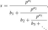
This gives rise to the continued fraction expansion of \(x \in {\mathcal {M}}\) in the form

(1)
where \(b_n \in k^{\times }, a_n \in {\mathbb {N}}\) for \(n=1,2,\ldots \). Here \({\mathbb {N}}\) denotes the set of natural numbers.
The rational approximants to \(x \in {\mathcal {M}}\) arise in a manner similar to that in the case of the real numbers as follows. We suppose \(A_0 = b_0, B_0=1, A_1 = b_0b_1+\pi ^{a_1}, B_1=b_1\). Then set
$$\begin{aligned} A_n=\pi ^{a_n}A_{n-2}+b_nA_{n-1} \ \text {and} \ B_n=\pi ^{a_n}B_{n-2}+b_nB_{n-1} \end{aligned}$$
(2)
for \(n\ge 2\). A simple inductive argument, for \(n=1,2, \ldots \) gives
$$\begin{aligned} A_{n-1}B_n-A_nB_{n-1} = (-1)^n\pi ^{a_1+\cdots +a_n}. \end{aligned}$$
(3)
The map \(T_v:{\mathcal {M}} \rightarrow {\mathcal {M}}\) preserves Haar measure on \({\mathcal {M}}\). By this we mean, for each Haar measurable set A contained in \({\mathcal {M}}\) we have \(\mu (T_v^{-1}(A))= \mu (A)\). Here \(T^{-1}_v(A) := \{ x\in {\mathcal {M}} : T_v(x)\in A \}\). To prove that \(T_v\) preserves Haar measure on \({\mathcal {M}}\) we only need to check it for special sets of the form \(\pi a + \pi ^n {\mathcal {O}}\), where \(a \in {\mathcal {O}}\). This is because sets of this form generate the Haar \(\sigma \)-algebra on \({\mathcal {M}}\). Suppose \(c_0 \in k\backslash \{ 0 \}\) and let m,n be positive integers. Then
$$\begin{aligned} T_v \left( \frac{\pi ^m}{c_0 + \pi a + \pi ^n {\mathcal {O}}} \right) = \pi a + \pi ^n {\mathcal {O}}. \end{aligned}$$
It follows
$$\begin{aligned} T_v ^{-1}(\pi a + \pi ^n {\mathcal {O}}) = \bigcup _{c_0 \in k\backslash \{0 \}} \bigcup _{m=1}^{\infty } \left( \frac{\pi ^m}{c_0 + \pi a + \pi ^n {\mathcal {O}}} \right) . \end{aligned}$$
Since
$$\begin{aligned} \frac{\pi ^m}{c_0 + \pi a + \pi ^n {\mathcal {O}}} = \frac{\pi ^m}{c_0 + \pi a} + \pi ^{n+m}{\mathcal {O}}, \end{aligned}$$
which has measure \(\# (k)^{1-m-n}\). Recall here \(\# (A)\) denotes the cardinality of the finite set A. It follows
$$\begin{aligned} \mu ( T_v ^{-1}(\pi a + \pi ^n {\mathcal {O}}))= & {} \sum _{c_0 \in k\backslash \{0 \}} \sum _{m=1}^{\infty } \mu \left( \frac{\pi ^m}{c_0 + \pi a} + \pi ^{n+m}{\mathcal {O}} \right) , \\= & {} \sum _{c_0 \in k\backslash \{0 \}} \sum _{m=1}^{\infty } \mu \left( \pi ^{n+m}{\mathcal {O}} \right) , \\= & {} \sum _{c_0 \in k\backslash \{0 \}} \sum _{m=1}^{\infty } \# (k )^{1-n-m}, \\= & {} \# (k)^{1-n} = \mu (\pi + \pi ^n {\mathcal {O}}), \end{aligned}$$
as required. So, \(T_v\) preserves Haar measure on \({\mathcal {M}}\).
In the case where \(K= {\mathbb {Q}}_p\) the map \(T_v\) reduces to the original Schneider's continued fraction map \(T_p\), which motivates this whole investigation and is defined as follows. For \(x \in p{\mathbb {Z}}_p\) define the map \(T_p: p{\mathbb {Z}}_p \rightarrow p{\mathbb {Z}}_p\) by
$$\begin{aligned} T_p(x)=\frac{p^{v(x)}}{x}-\left( \frac{p^{v(x)}}{x}\,\text{ mod }\;p \right) = \frac{p^{a(x)}}{x}-b(x), \end{aligned}$$
(4)
where v(x) is the p-adic valuation of x, \(a(x) \in {\mathbb {N}}\) and \(b(x) \in \{1,2,\ldots ,p-1\}\). Then using the continued fraction algorithm for x we get the expansion,
(5)
where \(b_n \in \{ 1,2, \ldots , p-1 \} , a_n \in {\mathbb {N}}\) for \(n=1,2,\ldots .\)
We now define the measure-theoretic entropy. Let \((X,{\mathcal {A}},m)\) be a probability space where X is a set, \({\mathcal {A}}\) is a \(\sigma \)-algebra of its subsets and m is a probability measure. A partition of \((X,{\mathcal {A}},m)\) is defined as a denumerable collection of elements \(\alpha =\{A_1,A_2,\ldots \}\) of \({\mathcal {A}}\) such that \(A_i\cap A_j=\emptyset \) for all \(i,j \in \Lambda \) with \( i\ne j\) and \(\bigcup _{i\in \Lambda }A_i=X.\) Here \(\Lambda \) is a denumerable index set. For a measure-preserving transformation T, we have \(T^{-1}\alpha =\{T^{-1}A_i|A_i\in \alpha \}\) which is also a denumerable partition. Given partitions \(\alpha =\{A_1,A_2,\ldots \}\) and \(\beta =\{B_1,B_2,\ldots \}\), we define the join of \(\alpha \) and \(\beta \) to be the partition \(\alpha \vee \beta =\{A_i\cap B_j|A_i\in \alpha ,B_j\in \beta \}.\) For a finite partition \(\alpha =\{A_1,\ldots ,A_n\}\), we define its entropy \(H(\alpha ):=-\sum _{i=1}^{n}m(A_i)\log m(A_i).\) Let \(\mathcal {A'}\subset {\mathcal {A}}\) be a sub-\(\sigma \)-algebra. Then we define the conditional entropy of \(\alpha \) given \({\mathcal {A}}'\) to be \(H(\alpha |\mathcal {A'}):=-\sum _{i=1}^{n}m(A_i|\mathcal {A'})\log m(A_i|\mathcal {A'})\). Here \(m (A| \mathcal {A'})\) denotes the m-conditional probability of A with respect to the \(\sigma \)-algebra \(\mathcal {A'}\). See [22] for more details about conditional probability. The entropy of a measure-preserving transformation T relative to a partition \(\alpha \) is defined to be
$$\begin{aligned} h_m(T,\alpha )=\lim _{n\rightarrow \infty } \frac{1}{n}H\left( \bigvee _{i=0}^{n-1}T^{-i}\alpha \right) , \end{aligned}$$
where the limit always exists. The alternative formula for \(h_m(T,\alpha )\) which is used for calculating entropy is
$$\begin{aligned} h_m(T,\alpha )=\lim _{n\rightarrow \infty }H\left( \alpha |\bigvee _{i=1}^{n}T^{-i}\alpha \right) =H \left( \alpha |\bigvee _{i=1}^{\infty }T^{-i}\alpha \right) . \end{aligned}$$
(6)
We define the measure-theoretic entropy of T with respect to the measure m to be \(h_m(T)=\sup _{\alpha }h_m(T,\alpha )\). Here the supremum is taken over all finite or countable partitions \(\alpha \) from \({\mathcal {A}}\) with \(H(\alpha )<\infty \).
Two measure-preserving transformations \((X_1 , \beta _1 , m_1, T_1 )\) and \((X_2, \beta _2, m_2 , T_2 )\) are said to be isomorphic if there exist sets \(M_1 \subseteq X_1\) and \(M_2 \subseteq X_2\) with \(m_1(M_1) =1\) and \(m_2(M_2) =1\) such that \(T_1(M_1) \subseteq M_1\) and \(T_2(M_2) \subseteq M_2\) and such that there exists a map \(\phi : M_1 \rightarrow M_2\) satisfying \(\phi T_1(x) = T_2\phi (x)\) for all \(x \in M_1\) and \(m_1(\phi ^{-1}(A)) = m_2(A)\) for all \(A \in \beta _2\). The importance of measure theoretic entropy is that two dynamical systems with different entropies can not be isomorphic. For more on measure-theoretic entropy and isomorphism, see [31]. The following is our first result.
Theorem 1.1
Let \({\mathcal {B}}\) denote the Haar \(\sigma \)-algebra restricted to \({\mathcal {M}}\) and let \(\mu \) denote the Haar measure on \({\mathcal {M}}\). Then the measure-preserving transformation \(( {\mathcal {M}} , {\mathcal {B}}, \mu , T_v) \) has measure-theoretic entropy \(\frac{\# (k)}{\# (k^{\times })}\log ( \# (k)).\)
The measure-preserving transformation \((p {\mathbb {Z}}_p , {\mathcal {B}}, \mu , T_p)\) is known to be ergodic [14]. Moreover, in [12] it was proved that \((p {\mathbb {Z}}_p , {\mathcal {B}}, \mu , T_p)\) is exact. We forgo the definition of exactness here, however, as we do not use the concept in this paper. The exactness of \((p {\mathbb {Z}}_p , {\mathcal {B}}, \mu , T_p)\) implies other weaker properties including mixing, which implies weak-mixing implying ergodicity, all implications being strict. Suppose \((Y, \alpha , l )\) is a probability space, and let \(Y_n =(Y, \alpha , l )\) for each \(n \in {\mathbb {Z}}\). Set \((X, \beta , m) = \Pi _{n\in {\mathbb {Z}}}Y_n\), i.e. the bi-infinite product probability space. For the shift map \(\tau (\{ x_n\} ) = (\{x_{n+1} \} )\), the measure-preserving transformation \((X, \beta , m, \tau )\) is called the Bernoulli process with state space \((Y, \alpha , l )\). Here \(\{ x_n \}\) is a bi-infinite sequence of elements of the set Y. Any measure-preserving transformation isomorphic to a Bernoulli process will be referred to as Bernoulli. The fundamental fact about Bernoulli processes, famously proved by D. Ornstein, is that Bernoulli processes with the same entropy are isomorphic [27]. To any measure-preserving transformation, \((X, \beta , m, T_0 )\) we can associate another called its natural extension. Originally introduced by V. A. Rokhlin [24], the natural extension is defined as follows. Set
$$\begin{aligned} X_{T_0} = \{ (x_0, x_1, x_2, \ldots ) : x_n =T_0 (x_{n+1}), x_n \in X , n=0,1,2, \ldots \} , \end{aligned}$$
and let \(T: X_{T_0} \rightarrow X_{T_0}\) be defined by
$$\begin{aligned} T(( x_0, x_1, \ldots , )) = ( T_0(x_0), x_0, x_1, \ldots , ). \end{aligned}$$
The map T is \(1-1\) on \(X_{T_0}\). If \(T_0\) preserves a measure m, then we can define a measure \({\overline{m}}\) on \(X_{T_0}\), by defining \({\overline{m}}\) on the cylinder sets
$$\begin{aligned} C(A_0, A_1, \ldots , A_k) = \{ \{ x_n \} :x_0\in A_0 , x_1 \in A_1, \ldots , x_k \in A_k \} \end{aligned}$$
by
$$\begin{aligned} {\overline{m}} (C(A_0, A_1, \ldots , A_k)) =m(T_0^{-k}(A_0) \cap T_0^{-k+1}(A_1) \cap \ldots \cap A_k) , \end{aligned}$$
for \(k\ge 1\). One can check that the transformation \((X_{T_0}, {\overline{\beta }}, {\overline{m}}, T_0)\) is measure-preserving as a consequence of the measure preservation of the transformation \((X, \beta , m, T_0)\). Our second theorem is the following.
Theorem 1.2
Suppose \(({\mathcal {M}} , {\mathcal {B}}, \mu , T_v) \) is as in our first theorem. Then the dynamical system \(( {\mathcal {M}} , {\mathcal {B}}, \mu , T_v) \) has a natural extension that is Bernoulli.
In last two sections of this paper, this theorem is combined with subsequence pointwise ergodic theorems and the moving average ergodic theorem [4], respectively, to study the average behaviour of the convergents arising from the map \(T_v\). These results in the special case \(K={\mathbb {Q}}_p\) already appear in [12]. Our two theorems above together tell us that as a dynamical system, the isomorphism class to which \(T_v\) belongs is determined solely by its residue class field. This is irrespective of the characteristic of the underlying global field. For instance, for each rational prime p the corresponding Schneider map has entropy \(\frac{p}{p-1} \log (p)\), so we know these maps are mutually non-isomorphic. Each of them is, however, isomorphic to the analogue of the Schneider map on the field of formal power series with coefficient field the finite field of p elements.
Henceforth, for a real number y let \(\{ y \}\) denote the fractional part of y. The study of the properties of \(( {\mathcal {M}} , {\mathcal {B}}, \mu , T_v)\) parallels that of the Gauss map defined on [0, 1] by
$$\begin{aligned} Tx = {\left\{ \begin{array}{ll} \left\{ { 1\over x } \right\} &{} \text { if} \ x \not = 0 ; \\ 0 &{} \ \text {if} \ x=0. \end{array}\right. } \end{aligned}$$
This map preserves the measure defined for Lebesgue measurable \(A\subseteq [0,1]\) by
$$\begin{aligned} \eta (A) \ = \ {1\over \log 2}\int _A {\mathrm{d}x \over x+1}. \end{aligned}$$
Like \(( {\mathcal {M}} , {\mathcal {B}}, \mu , T_v)\), if \({\mathcal {L}}\) denotes the Lebesgue \(\sigma \)-algebra on [0, 1], the transformation \(([0,1], {\mathcal {L}}, \eta , T)\) also has a Bernoulli natural extension and in this case has entropy \(\frac{\pi ^2}{6\log (2)}\). Evidently the Gauss map cannot be isomorphic to \(( {\mathcal {M}} , {\mathcal {B}}, \mu , T_v)\), for any v.
Analogously to the Gauss map [13], the map which governs the regular continued fraction on the real numbers, the measure-preserving transformation \(( p{\mathbb {Z}}_p , {\mathcal {B}}, \mu , T_p)\) via (4) gives rise to an integer recurrence relationship. This is as follows. We Suppose \(A_0 = b_0, B_0=1, A_1 = b_0b_1+p^{a_1}, B_1=b_1\). Then set
$$\begin{aligned} A_n=p^{a_n}A_{n-2}+b_nA_{n-1} \ \text {and} \ B_n=p^{a_n}B_{n-2}+b_nB_{n-1} \end{aligned}$$
(7)
for \(n\ge 2\). A simple inductive argument gives for \(n=1,2, \ldots \).
$$\begin{aligned} A_{n-1}B_n-A_nB_{n-1} = (-1)^np^{a_1+\ldots +a_n}. \end{aligned}$$
(8)
Because p does not divide \(B_n\) we deduce that the integers \(A_n\) and \(B_n\) are coprime. The sequence of rationals \(({A_n\over B_n})_{n=1}^{\infty }\) are the convergents to x in \(p{{\mathbb {Z}}}_p\) arising from (5). Naturally one of the first things one might try to do is explore the extent to which, theorems true for continued fractions on the real numbers extend to the p-adic numbers. For the most part, one can extend the regular continued fraction expansion and its properties to the field of formal Laurent series over a finite field, in a relatively trouble-free manner. This is primarily because the field of formal Laurent series over a finite field is a Euclidean domain. In the context of the p-adic numbers the direct analogue of the regular continued fraction is the Ruban continued fraction [25]. Here, however, there are problems. The p-adic numbers are not a Euclidean domain. It is possible to define a sequence of rationals analogous to the convergents of the regular continued fractions. Their convergence to the number they are supposed to represent is not assured, however. This problem can be got round using a system of weights. This is what leads to Schneider's continued fraction expansion. This is at a cost, however. Some partial success at recovering analogues of standard properties of the regular continued fraction for the real numbers is possible on the p-adic numbers. See, for instance, [1,2,3, 8, 11], where the issues of when a p-adic continued fraction is either finite or periodic is explored. One cannot, however, hope to have a theory as satisfactory or as useful as that offered by the regular continued fraction expansion. The situation is just more complex. For instance, unlike the sequence of convergents of the regular continued fraction expansion, the sequence \(({A_n\over B_n})_{n=1}^{\infty }\) does not always provide a sequence of best approximants to the p-adic number they approximate. Other solutions to this particular problem are available, though not using Schneider's map however [20, 21]. All this said, as observed in [7], while not as versatile as the regular continued fraction, Schneider continued fraction can be a powerful tool in a number of situations. It is sometimes very useful in delicate constructions on the p-adic numbers. In [7] for instance it is used to construct numbers that distinguish between the Mahler and Koksma schemes of approximation to a specified degree. Specifically for a p-adic number \(\eta \) let w(n) denote its Mahler function on \({{\mathbb {N}}}\) defined to be the supremum of all real numbers w such that the inequality
$$\begin{aligned} 0< |P(\eta ) |_p \le H(P)^{-w-1} \end{aligned}$$
is satisfied by infinitely many polynomials P over \({\mathbb {Z}}\) of degree at most n. Here H denotes the height of the polynomial P, defined to be the maximum of the absolute values of the coefficients of P. Analogously, to \(\eta \) we can also associate the Koksma function \(w^*(n)\) which is defined to be the supremum over all real numbers w such that the inequality
$$\begin{aligned} 0< |\eta - \xi |_p \le H(\xi )^{-w-1} \end{aligned}$$
is satisfied by infinitely many algebraic numbers \(\xi \) of degree at most n. In this instance \(H(\xi )\) denotes the height of the minimal polynomial defining \(\xi \). The relationship between the numbers w(n) and \(w^*(n)\) is a complex and unresolved issue. Restricting to the case \(n=2\) some progress has been made, though even here this is not an easy matter. It is known \(w(2) \in [w^*(2), w^*(2)+1]\). We also know that \(w(2) = w^*(2)\) for almost all \(\eta \) in \({\mathbb {Q}}_p\). Methods of diophantine approximation have been used to show there are p-adic numbers \(\eta \) such that \(w(2)= w^*(2) +\delta \) for each \(\delta \in [0,1)\). Constructing \(\xi \) such that \(w(2)= w^*(2)+1\) has so for only proved possible using the Schneider continued fraction. The method has the additional advantage over diophantine approximation methods of being constructive. The details of this are to be found in [7]. See also [5, 6] for related applications.
Another interesting application of Schneider's continued fraction is to deciding the algebraic independence of a set of p-adic numbers. See [9, 19] for details.
For background on the theory of regular continued fractions and its ergodic theory see for instance [13, 15]. As is well known, if you restrict the Gauss map to the rational numbers you get the Euclidean algorithm. If you set \(p=2\) and restrict the Schneider map to the rational numbers what you get is the Binary Euclidean algorithm. This is another way of calculating the highest common factor of two integers, particularly well adapted to efficient implementation on binary machines. The algorithm was first published by Josef Stein [29] but is also attributed to Roland Silver and John Terzian in unpublished form [17]. The algorithm may, however, be much older. Knuth [17] cites a verbal description of the algorithm in the first-century A.D. Chinese text "Chiu Chang Suan Shu".
The Entropy of Schneider's Continued Fraction Map
In this section, we will prove the first result of the paper.
One can see that it can be complicated to compute entropy from its definition, so there is the following theorem due to Ya. G. Sinai which is the main tool. The proof of the theorem and more information about entropy can be found in Chapter 4 of [31].
Theorem 2.1
If \(\alpha \) is a strong generator, i. e. \(\bigvee _{i=0}^{n-1}T^{-i}\alpha \rightarrow {\mathcal {A}}\) as \(n\rightarrow \infty ,\) and if \(H(\alpha )<\infty \) then
$$\begin{aligned} h_m(T)=h_m(T,\alpha ). \end{aligned}$$
Proof of Theorem 1.1
Let \(B = k^{\times }\times {\mathbb {N}}\) and let \(j=(j_1,j_2,\ldots )\) be a countable sequence of elements of B. For a particular element \(j^* =(b, a) \in B\), define the cylinder-set \(\Delta (j^*)\) by
$$\begin{aligned} \Delta (j^*)=\left\{ x\in {\mathcal {M}} :v(x)=a \text { and } \left( \frac{\pi ^{v(x)}}{x}\mod \pi \right) =b \right\} . \end{aligned}$$
Now let \(\Delta ^{(0)}= {\mathcal {M}}\) and let \(\Delta ^{(1)}_{j}= \Delta (j_1)\), where \(j_1\) is the first element of the sequence j. Next define
$$\begin{aligned} \Delta ^{(2)}_j= \{ x\in {\mathcal {M}} :x\in \Delta (j_1) \text { and } T_v(x)\in \Delta (j_2) \}. \end{aligned}$$
Proceeding inductively, we get
$$\begin{aligned} \Delta ^{(n)}_{j}= \{ x\in {\mathcal {M}} :x\in \Delta (j_1), T_v(x)\in \Delta (j_2),\ldots , T_v^{n-1}(x)\in \Delta (j_n) \}. \end{aligned}$$
So, \(\Delta ^{(n)}_{j}\) is the set of all \(x \in {\mathcal {M}}\) with continued fraction expansion starting with \(j_1,j_2,\ldots ,j_n\). This means that \(\Delta ^{(n)}_{j}\) depends only on the first n terms of j. If \(J_n =(j_1,j_2,\ldots ,j_n)\in B^n\), we have
$$\begin{aligned} {\mathcal {M}}= \bigcup _{J_n\in B^n} \Delta ^{(n)}_{j} \quad \text { for all}\quad ~ n\ge 1 \end{aligned}$$
such that
$$\begin{aligned} \bigcup _{j_n\in B} \Delta ^{(n)}_j= & {} \Delta ^{(n-1)}_j \\ T_v( \Delta ^{(n)}_j)= & {} \Delta ^{(n-1)}_j \end{aligned}$$
and
$$\begin{aligned} T_v(\Delta ^{(1)}_{j})= {\mathcal {M}}. \end{aligned}$$
Now take \(j_n=(b_n,a_n), n=1,2,\ldots \) with \(j_r \not = j_s\) if \(r \not = s\) and let \(\alpha =\{\Delta (j_1),\Delta (j_2),\Delta (j_3),\ldots \}\) be the partition. Notice that
$$\begin{aligned} \Delta ^{(n)}_{j}= & {} \Delta (j_1) \cap T_v^{-1}(\Delta ( j_2)) \cap T_v^{-2}(\Delta (j_3))\cap \cdots \cap T_v^{-(n-1)}(\Delta (j_n)) \\= & {} \Delta _j^{(1)} \cap \bigcup _{J_1\in B}\Delta ^{(2)}_j \cap \bigcup _{J_2\in B^2}\Delta ^{(3)}_j \cap \cdots \cap \\&\bigcup _{J_{n-1}\in B^{n-1}} \Delta ^{(n)}_j. \end{aligned}$$
To compute entropy, we first need to find the conditional information function \(I(\alpha |\bigvee _{i=1}^{n-1}T_v^{-i}\alpha )\) which is defined as
$$\begin{aligned} I(\alpha |T_v^{-1}\alpha \vee \cdots \vee T_v^{-(n-1)}\alpha )=-\sum _{\Delta (j)\in \alpha }\chi _{\Delta (j)}(x)\log \mu (\Delta (j)|T_v^{-1}\alpha \vee \cdots \vee T_v^{-(n-1)}\alpha ). \end{aligned}$$
Here, for a partition \(\phi \) the symbol \(\mu (A| \phi )\) denotes the \(\mu \)-conditional probability of A with respect to the \(\sigma \)-algebra generated by the partition \(\phi \). If \(x \in \Delta ^{(n)}_{j}\), then \(\chi _{\Delta (j_1)}(x)=1\) and \(\chi _{\Delta (j_i)}(x)=0\) for all \(i\ge 2.\) So we get
$$\begin{aligned} I(\alpha |T_v^{-1}\alpha \vee \cdots \vee T_v^{-(n-1)}\alpha )=-\log \mu (\Delta (j_1)|T_v^{-1}\alpha \vee \cdots \vee T_v^{-(n-1)}\alpha ). \end{aligned}$$
The conditional probability is
$$\begin{aligned} \mu (\Delta (j_1)|T_v^{-1}\alpha \vee \cdots \vee T_v^{-(n-1)}\alpha )=\sum _{C\in T_v^{-1}\alpha \vee \cdots \vee T_v^{-(n-1)}\alpha }\chi _C(x)\frac{\mu (\Delta (j_1)\cap C)}{\mu (C)}. \end{aligned}$$
If \(x \in \Delta ^{(n)}_{j}\), we set \(C_1=T_v^{-1}(\Delta (j_2))\cap T_v^{-2}(\Delta (j_3))\cap \cdots \cap T_v^{-(n-1)}(\Delta (j_n))\). Then we can see that \(\chi _{C_1}(x)=1\) and for other
$$\begin{aligned} C_i\ne T_v^{-1}(\Delta (j_2))\cap \cdots \cap T_v^{-(n-1)}(\Delta (j_n)), \end{aligned}$$
where \(i\ge 2\) we have \(\chi _{C_i}(x)=0.\) Thus, we obtain
$$\begin{aligned}&\mu (\Delta (j_1)|T_v^{-1}\alpha \vee \cdots \vee T_v^{-(n-1)}\alpha ) \\&\quad =\frac{\mu (\Delta (j_1)\cap T_v^{-1}(\Delta (j_2))\cap \cdots \cap T_v^{-(n-1)}(\Delta (j_n)))}{\mu ( T_v^{-1}(\Delta (j_2))\cap \cdots \cap T_v^{-(n-1)}(\Delta (j_n)))} \\&\quad = \frac{\mu (\Delta ^{(n)}_j)}{\mu (\Delta ^{(n-1)}_j)}. \end{aligned}$$
A simple computation shows that \(\mu (\Delta ^{(n)}_{j})=\frac{1}{\# (k)^N}\), where \(N=a_1+a_2+\cdots +a_n.\) Thus, we have
$$\begin{aligned} \mu (\Delta (j_1)|T_v^{-1}\alpha \vee \cdots \vee T_v^{-(n-1)}\alpha )=\left. \frac{1}{\# (k)^N} \big / \frac{1}{\# ( k )^{N-a_1}}\right. =\# ( k )^{-a_1} \end{aligned}$$
and the conditional information function is
$$\begin{aligned} I(\alpha |T_v^{-1}\alpha \vee \cdots \vee T_v^{-(n-1)}\alpha )=-\log ( \# (k)^{-a_1})=a_1\log ( \# (k) ) . \end{aligned}$$
By (6), we see that the entropy of \(T_v\) relative to the partition \(\alpha \) is
$$\begin{aligned} h_{\mu }(T_v,\alpha )=\lim _{n\rightarrow \infty }H\left( \alpha |\bigvee _{i=1}^{n-1}T_v^{-i}\alpha \right) , \end{aligned}$$
where
$$\begin{aligned} H\left( \alpha |\bigvee _{i=1}^{n-1}T_v^{-i}\alpha \right) =\int {I\left( \alpha |\bigvee _{i=1}^{n-1}T_v^{-i}\alpha \right) }\mathrm{d}\mu . \end{aligned}$$
So, we get
$$\begin{aligned} h_{\mu }(T_v,\alpha )=\lim _{n\rightarrow \infty }\int {a_1\log ( \# (k)}) \;\mathrm{d}\mu . \end{aligned}$$
Notice that \(a_1(x)=v(x)\) and we have
$$\begin{aligned} h_{\mu }(T_v,\alpha )=\lim _{n\rightarrow \infty }\int {v(x)\log ( \# ( k ))}\;\mathrm{d}\mu =\frac{\# ( k )}{\# ( k^{\times } )}\log ( \# (k)). \end{aligned}$$
We claim that \(\alpha \) is a strong generator for \(T_v\). This is because for almost every \(x,y \in {\mathcal {M}}\) if \(x\ne y\), the points x and y have distinct Schneider continued fraction expansions. This implies the partition \(\alpha \) separates almost every pair of points. Hence, by Sinai's Theorem 2.1, the entropy of \(T_v\) with respect to \(\mu \) is
$$\begin{aligned} h_{\mu }(T_v)=h_{\mu }(T_v, \alpha )=\frac{\# (k) }{\# (k^{\times }) }\log ( \# (k)). \end{aligned}$$
\(\square \)
Proof of the Bernoulli Property
Let \(P=(p_1, p_2,\ldots )\) and \(Q=(q_1,q_2,\ldots )\) denote two \(\mu \)-measurable denumerable partitions of the same set X. Then P and Q are said to be \(\varepsilon \)-independent and we write \(P \bot ^{\varepsilon } Q\) if
$$\begin{aligned} \sum _i \sum _j |\mu (p_i \cap q_j)-\mu (p_i)\mu (q_j)|<\varepsilon . \end{aligned}$$
A denumerable partition P is called weak Bernoulli with respect to an invertible, measure-preserving transformation T if for each \(\varepsilon >0\) there exists a positive constant \(K=K(\varepsilon )\) such that for every \(n\ge 0\) we have
$$\begin{aligned} \bigvee _{i=-n}^{0}T^iP \; \bot ^{\varepsilon } \,\bigvee _{i=K}^{K+n} T^iP. \end{aligned}$$
Note this is not the only way to formulate this property. As observed in [28] for a non-invertible transformation, its natural extension is weakly Bernoulli, if there is a denumerable partition such that for each \(\varepsilon >0\) there exists \(K=K(\varepsilon )\) and every \(n\ge 0\) we have
$$\begin{aligned} \bigvee _{i=0}^{n}T^{-i}P \; \bot ^{\varepsilon } \,\bigvee _{i=K+n}^{K+2n} T^{-i}P. \end{aligned}$$
The isomorphism to a Bernoulli shift is then ensured by the following theorem which was proved by Friedmann and Ornstein, see [27].
Theorem 3.1
A weak Bernoulli (invertible) transformation is isomorphic to a Bernoulli shift with the same entropy.
We now complete the proof of our second theorem.
Proof of Theorem 1.2
Set
$$\begin{aligned} A_{j}=T_v^{-n-l}(A)\cap \Delta ^{(n)}_j \end{aligned}$$
then we get
$$\begin{aligned} \mu (A_{j})=\int _{T_v^{-l}A} \frac{\mathrm{d}\mu (T_v^{-n}(x))}{\mathrm{d}\mu (x)}\mathrm{d}\mu (x)=\int _{T_v^{-l}A} \mathrm{d}\mu (T_v^{-n}(x)). \end{aligned}$$
Lemma 3.1
\(\mathrm{d}\mu (T_v^{-n}(x))=\frac{1}{\# (k )^N}\mathrm{d}\mu (x)\) where \(N=a_1+ \cdots + a_n\) (on \(\Delta ^{(n)}_{j}\)).
Proof
For \(x \in \Delta ^{(n)}_{j}\), suppose its \(n^{th}\) convergent is \(\frac{A_n}{B_n}\) defined by the recurrence relation (4) . Using (4) and (5) one checks that
$$\begin{aligned} T^{-n}_v(x) =\frac{xA_{n-1}+B_n}{xB_{n-1}+B_n} = \frac{A_n}{B_n} + \frac{(-1)^nx\pi ^N}{(xB_{n-1}+B_n)B_n}. \end{aligned}$$
As \(B_n\) is in \({\mathcal {O}}^{\times }\) and multiplication by \(\pi ^N\) scales Haar measure by \(|\pi |^{-N}\), this lemma is proved if we show that the map \(t: {\mathcal {M}} \rightarrow {\mathcal {M}}\) defined by \(t(x) =\frac{x}{xB_{n-1}+B_n}\) preserves Haar measure. Fix \(L\in {{\mathbb {N}}}\) and \(y \in k[ \pi ]\) (the ring of polynomials in \(\pi \) over the residue class ring). One checks readily that t maps the coset \(\pi y+\pi ^L{\mathcal {O}}\) bijectively to the coset \(t(\pi y)+\pi ^L{\mathcal {M}}\). Cosets of this type form a basis for the open sets of \({\mathcal {M}}\) and have the same measure, so their measure is preserved. Hence, our lemma is proved. \(\square \)
We, therefore, have
$$\begin{aligned} \mu (A_{j})=\frac{1}{\# (k)^N}\int _{T_v^{-l}A} \mathrm{d}\mu (x)=\frac{1}{\# (k)^N}\mu (T_v^{-l}A)=\frac{1}{\# (k)^N}\mu (A). \end{aligned}$$
Recall that \(\frac{1}{\# (k)^N}=\mu (\Delta ^{(n)}_j).\) So we get
$$\begin{aligned} \mu (T_v^{-n-l}(A)\cap \Delta ^{(n)}_{j})=\mu (\Delta ^{(n)}_{j})\mu (A). \end{aligned}$$
Suppose both \(\Delta ^{(n)}(j)\) and A belong to \(\bigvee _{i=0}^{n}T_v^{-i}\alpha \), where
$$\begin{aligned} \alpha =\{\Delta (j_1),\Delta (j_2),\Delta (j_3),\ldots \} \end{aligned}$$
is a generator for \(T_v.\) Then \(\Delta =T_v^{-l-n}A \in \bigvee _{i=k+n}^{k+2n} T_v^{-i}\alpha \) and we get
$$\begin{aligned} \mu (\Delta \cap \Delta ^{(n)}_{j})-\mu (\Delta )\mu (\Delta ^{(n)}_{j})=0 \end{aligned}$$
which implies
$$\begin{aligned} \sum _{\Delta ^{(n)}_{j}\in \bigvee _{i=0}^{n}T_v^{-i}\alpha }\sum _{\Delta \in \bigvee _{i=k+n}^{k+2n} T_v^{-i}\alpha } { \left| \mu (\Delta \cap \Delta ^{(n)}_{j})-\mu (\Delta )\mu (\Delta ^{(n)}_{j})\right| }=0<\varepsilon . \end{aligned}$$
Thus, the generator \(\alpha \) for \(T_v\) is weak Bernoulli which by the above theorem means that the natural extension of \(T_v\) is isomorphic to a Bernoulli shift with the entropy \(\frac{\# (k)}{\# (k^{\times })}\log ( \# (k)).\) \(\square \)
Application of the Pointwise Subsequence Ergodic Theorems
Recall the elementary identities \(\sum _{n=1}^\infty nx^{n}= \frac{x}{(1-x)^2} \) and \(\sum _{n=1}^\infty n^2x^{n}= \frac{1+x}{(1-x)^3}\) for \(|x| < 1\). Also as is easily verified
$$\begin{aligned} \mu ( \{ x: v(x)=n\} ) = \frac{\# (k^{\times })}{\# (k)^n} \quad (n=1,2, \ldots ). \end{aligned}$$
From this, we get
$$\begin{aligned} \int _{{\mathcal {M}}}v(x) \mathrm{d}\mu (x)= \sum _{n=1}^\infty n \mu ( \{ x: v(x)=n\} ) = \frac{\# (k) }{\# (k^{\times })} \end{aligned}$$
and
$$\begin{aligned} \int _{ {\mathcal {M}}}|v(x)|^2 \mathrm{d}\mu (x)= \sum _{n=1}^\infty n^2 \mu ( \{ x: v(x)=n\} ) = \frac{\# (k)^2(\# (k)+1)}{\# (k^{\times })^2}. \end{aligned}$$
We now describe the elements of subsequence ergodic theory, which we use to study convergents.
A sequence of integers \((a_n)_{n=1}^{\infty }\) is called \(L^p\)-good universal if for each dynamical system \((X,{\mathcal {B}}, \mu ,T)\) and \(f\in L^p(X,{\mathcal {B}}, \mu )\), we have
$$\begin{aligned} {{\overline{f}}}(x)=\lim _{N\rightarrow \infty } \frac{1}{N} \sum _{n=1}^N f( T^{a_n}x) \qquad \text {existing}~ \mu ~\text {almost everywhere.} \end{aligned}$$
Recall that we say a sequence of real numbers \((x_n)_{n=1}^{\infty }\) is uniformly distributed modulo one if for each interval \(I \subseteq [0,1)\), denoting its length by |I|, we have
$$\begin{aligned} \lim _{N\rightarrow \infty }{1\over N} \#\{ n\le N : \{x_n \} \in I \} = |I|. \end{aligned}$$
See [18] for further background. The reference [12] contains an extensive list of sequences of natural numbers, that are \(L^p\)-good universal for all \(p>1\). Some are \(L^1\)-good universal as well. All the examples mentioned in the reference have the additional property that \((\{ k_n \psi \})_{n\ge 1}\) is uniformly distributed for each irrational number \(\psi \). We will call a sequence of natural numbers \((k_n)_{n\ge 1}\) that is both \(L^p\)-good universal and such that \(( \{ k_n \psi \} )_{n\ge 1}\) is uniformly distributed modulo one for each irrational \(\psi \) p-good. In [12], the following theorem is proved.
Theorem 4.1
If \((k_n)_{n\ge 1}\) is p-good for any \(p> 1\) and the dynamical system \((X, \beta , \mu , T)\) is weak-mixing, then \({{{\overline{f}}}}(x) = \int _Xf\mathrm{d}\mu \) \(\mu \) almost everywhere.
the following result.
Note that transformations that have natural extensions that are Bernoulli are also weak-mixing [31]. Theorem 4.1 has a number of applications.
Theorem 4.2
Suppose \((k_n)_{n\ge 1}\) is an p-good and suppose \(F: {{\mathbb {R}}}_{\ge 0} \rightarrow {{\mathbb {R}}}\) is a continuous increasing function with
$$\begin{aligned} \int _{{{\mathcal {M}}}}|F(a_1(x))|^p\mathrm{d}x < \infty . \end{aligned}$$
For each \(n \in {{\mathbb {N}}}\) and arbitrary real numbers \(d_1, \ldots , d_n\), we define
$$\begin{aligned} M_{F, n}(d_1, \ldots , d_n) = F^{-1}\left[ {F(d_1) + \cdots + F(d_n ) \over n } \right] . \end{aligned}$$
Then we have
$$\begin{aligned} \lim _{n\rightarrow \infty }M_{F,n}(a_{k_1}(x), \ldots , a_{k_n}(x)) = F^{-1}\left[ \int _{{\mathcal {M}}}F(a_1(x))\mathrm{d}x \right] \end{aligned}$$
almost everywhere with respect to Haar measure on \({\mathcal {M}}\).
Proof
Apply Theorem 4.1 with \(f(x) =F(a_1(x))\). \(\square \)
Theorem 4.3
For an p-good \((k_n)_{n\ge 1}\) and a function \(H : {{\mathbb {N}}}^m \rightarrow {{\mathbb {R}}}\), suppose that
$$\begin{aligned} \int _{{{\mathcal {M}}}}|H(a_1(x), \ldots , a_m(x))|^p \mathrm{d}x < \infty . \end{aligned}$$
Then we have
$$\begin{aligned} \lim _{N\rightarrow \infty }{1\over N} \sum _{n=1}^NH( a_{k_n}(x) , a_{k_n+1}(x), \ldots , a_{k_n+m}(x) ) = \sum _{i^{(m)} \in {\mathbb N}^m}H(i^{(m)}) \left( {\# (k^{\times })^m \over \# ( k)^{i_1+ \cdots +i_n}} \right) \end{aligned}$$
almost everywhere with respect to Haar measure on \({\mathcal {M}}\).
Proof
Apply Theorem 4.1 with \(f(x) =H(a_1(x), \ldots , a_m(x))\). \(\square \)
Theorem 4.4
For any p-good \((k_n)_{n\ge 1}\), we have
$$\begin{aligned} \lim _{N\rightarrow \infty }{1\over N} \sum _{n=1}^Na_{k_n} ={\# (k) \over \# ( k^{\times } )}, \end{aligned}$$
and
$$\begin{aligned} \lim _{N\rightarrow \infty }{1\over N} \sum _{n=1}^Nb_{k_n} ={\# (k^{\times })\over 2}, \end{aligned}$$
almost everywhere with respect to Haar measure on \({\mathcal {M}}\).
Proof
Apply Theorem 4.1 with \(f(x) =v(x)\) and \(f(x) = b(x)\). \(\square \)
In the case \(k_n=n \ (n=1,2, \ldots )\) and \(K= {\mathbb {Q}}_p\), the first part of this result is from [14]. Unlike the natural numbers, however, most examples of p-good sequences are of zero density. We also have the following additional consequences.
Theorem 4.5
For any p-good \((k_n)_{n\ge 1}\), we have
$$\begin{aligned} \lim _{N\rightarrow \infty }{1\over N} \# \{ 1 \le n \le N : a_{k_n} = i \}= & {} {\# (k^{\times } )\over \# ( k )^i}, \\ \lim _{N\rightarrow \infty }{1\over N} \# \{ 1 \le n \le N : a_{k_n} \ge i \}= & {} {1\over \# ( k )^i}, \end{aligned}$$
and
$$\begin{aligned} \lim _{N\rightarrow \infty }{1\over N} \# \{ 1 \le n \le N : i\le a_{k_n} < j \} ={1\over \# ( k )^{i+1}}\left( 1 -\left( {1\over \# (k )^{j-i-1}} \right) \right) ; \end{aligned}$$
almost everywhere with respect to Haar measure on \({\mathcal {M}}\).
Proof
Apply Theorem 4.1 with \(f(x) =I_{B_i}(x) \ (i=1,2,3)\), where \(I_B\) is the characteristic function of the set B in the cases
$$\begin{aligned} B_1= & {} \{ x \in {{\mathcal {M}}} : a_i(x) =i \}, \\ B_2= & {} \{ x \in {\mathcal {M}} : a_i(x) \ge i \} \end{aligned}$$
and
$$\begin{aligned} B_3 = \{ x \in {\mathcal {M}} : i\le a_i(x) < j \}. \end{aligned}$$
\(\square \)
Application of the Moving Average Pointwise Ergodic Theorem
We begin by introducing some notation. Let Z be a collection of points in \({{\mathbb {Z}}}\times {\mathbb {N}}\) and let
$$\begin{aligned} Z^h= & {} \{ (n,k) \ : \ (n,k) \ \in \ Z \mathrm{and} \ k \ \ge \ h \}, \\ Z^h_{\alpha }= & {} \{ (z,s) \ \in \ {{\mathbb {Z}}}^2 \ : \ |z \ - \ y| \ < \ \alpha (s \ - \ r) \mathrm{for some} \ (y,r) \ \in Z^h \} \end{aligned}$$
and
$$\begin{aligned} Z^h_{\alpha }(\lambda ) \ = \ \{ n : \ (n, \lambda ) \ \in \ Z^h_{\alpha } \}. \qquad ( \lambda \in {{\mathbb {N}}} ) \end{aligned}$$
Geometrically we can think of \(Z^1 _{ \alpha }\) as the lattice points contained in the union of all solid cones with aperture \(\alpha \) and vertex contained in \(Z^1= Z\). We say a sequence of pairs of natural numbers \((n_l ,k_l )_{l=1}^{\infty }\) is Stoltz if there exists a collection of points Z in \({{\mathbb {Z}}}\times {\mathbb {N}}\), and a function \(h = h(t)\) tending to infinity with t such that \((n_l,k_l )_{l=t}^{\infty } \ \in \ Z^{h(t)}\) and there exist \(h_0\), \(\alpha _0\) and \(A \ > \ 0\) such that for all integers \(\lambda \ > \ 0\) we have \(|Z^{h_0}_{\alpha _0}(\lambda )| \ \le \ A\lambda \). This technical condition is interesting because of the following theorem from [4].
Theorem 5.1
Let \((X,\beta ,\mu , T )\) denote a dynamical system, on set X, with a \(\sigma \)-algebra of its subsets \(\beta \), a measure \(\mu \) defined on the measurable space \((X,\beta )\) such that \(\mu (X) = 1\) and a measurable, measure-preserving map T from X to itself. Suppose f is in \(L^1(X,\beta , \mu )\) and that the sequence of pairs of natural numbers \((n_l , k_l)_{l=1}^{\infty }\) is Stoltz then if \((X, \beta , \mu , T)\) is ergodic, the limit
$$\begin{aligned} m_f(x) = \lim _{l\rightarrow \infty }{1\over k_l}\sum _{i=1}^{k_l}f(T^{n_l+i}x), \end{aligned}$$
exists almost everywhere with respect to Lebesgue measure.
Note that if we set
$$\begin{aligned} m_{l, f}(x) = {1\over k_l}\sum _{i=1}^{k_l}f(T^{n_l+i}x) \end{aligned}$$
then
$$\begin{aligned} m_{l,f}(Tx)- m_{l,f}(x) = k_l^{-1}(f(T^{n_l+k_l+1})- f(T^{n_l+1}x)). \end{aligned}$$
This means that \(m_f(Tx) = m_{f}(x)\) \(\mu \) almost everywhere. A standard fact in ergodic theory is that if \((X,\beta , \mu , T)\) is ergodic and \(m_f (Tx) = m_f(x)\) almost everywhere, then \(m_f(x) = \int _X f\mathrm{d}\mu \) \(\mu \) almost everywhere [31]. The term Stoltz is used here because the condition on \((k_l,n_l )_{l=1}^{\infty }\) is analogous to the condition required in the classical non-radial limit theorem for harmonic functions also called a Stoltz condition, which suggested the above theorem to the authors of [4]. Averages where \(k_l=1\) for all l will be called non-moving. Moving averages satisfying the above hypothesis can be constructed by taking for instance \(n_l=2^{2^l}\) and \(k_l=2^{2^{l-1}}\).
In this section, we state moving average variants of the results in the previous section. The proofs, which are very similar to those in the previous section, are forgone.
Theorem 5.2
Suppose that \((n_l, k_l)_{l\ge 1}\) is Stoltz. Suppose also that we have \(F: {{\mathbb {R}}}_{\ge 0} \rightarrow {{\mathbb {R}}}\) which is continuous increasing and such that
$$\begin{aligned} \int _{{\mathcal {M}}}|F(a_1(x))|\mathrm{d}x < \infty . \end{aligned}$$
Suppose \(M_{F, n}(d_1, \ldots , d_n)\) is defined as in the previous section. Then
$$\begin{aligned} \lim _{l\rightarrow \infty }M_{F,l}(a_{k_l}(x), \ldots , a_{k_l+n_l}(x)) = F^{-1}\left[ \int _{{\mathcal {M}}}F(a_1(x))\mathrm{d}x \right] \end{aligned}$$
almost everywhere with respect to Haar measure on \({\mathcal {M}}\).
Theorem 5.3
Suppose \((n_l, k_l)_{l\ge 1}\) is Stoltz and \(H : {{\mathbb {N}}}^m \rightarrow {{\mathbb {R}}}\) is such that
$$\begin{aligned} \int _{{\mathcal {M}}}|H(a_1(x), \ldots , a_m(x))| \mathrm{d}x < \infty . \end{aligned}$$
Then we have
$$\begin{aligned} \lim _{l\rightarrow \infty }{1\over {n_l}} \sum _{j=1}^{n_l}H( a_{k_l+1+j}, a_{k_l+2+j}, \ldots , a_{k_l+m+j} )(x) = \sum _{i^{(m)} \in {\mathbb N}^m}H(i^{(m)}) \left( {\# (k^{\times })^m \over \# (k )^{i_1+ \cdots +i_m}} \right) \end{aligned}$$
almost everywhere with respect to Haar measure on \({\mathcal {M}}\).
Theorem 5.4
Suppose \((k_l,n_l)_{n\ge 1}\) is Stoltz then we have
$$\begin{aligned} \lim _{l\rightarrow \infty }{1\over n_l} \sum _{j=1}^{n_l}a_{k_l+j } ={\# (k) \over \# (k^{\times })}, \end{aligned}$$
and
$$\begin{aligned} \lim _{l\rightarrow \infty }{1\over n_l} \sum _{j=1}^{n_l}b_{k_l+j} ={\# ( k^{\times } )\over 2}, \end{aligned}$$
almost everywhere with respect to Haar measure on \({\mathcal {M}}\).
Theorem 5.5
For Stoltz \((n_l, k_l)_{l \ge 1}\), we have
$$\begin{aligned} \lim _{l\rightarrow \infty }{1\over n_l} \# \{ 1 \le j \le n_l : a_{k_l+j}= & {} i \} ={\# (k^{\times })\over \# (k)^i}, \\ \lim _{l\rightarrow \infty }{1\over n_l} \# \{ 1 \le j \le n_l : a_{k_l+j} \ge i \}= & {} {1\over \# (k)^i}, \end{aligned}$$
and
$$\begin{aligned} \lim _{l\rightarrow \infty }{1\over n_l} \# \{ 1 \le t \le n_l : i\le a_{k_l+t} < j \} ={1\over \# (k)^{i+1}}\left( 1-\left( {1\over \# (k)^{j-i-1}} \right) \right) , \end{aligned}$$
almost everywhere with respect to Haar measure on \({\mathcal {M}}\).
References
-
Becker, P.G.: Periodizitätseigenschaften p-adischer Kettenbrüche, (German) [Periodicity properties of p-adic continued fractions] Elem. Math. 45(1), 1–8 (1990)
-
E. Bedocchi: A note on p-adic continued fractions, (Italian) Ann. Mat. Pura Appl. (4) 152 (1988), 197–207
-
Bedocchi, E.: Sur le développement de \(\sqrt{m}\) en fraction continue p-adique. (French) [On the expansion of \(\sqrt{m}\) into a p-adic continued fraction]. Manuscr. Math. 67(2), 187–195 (1990)
-
Bellow, A., Jones, R., Rosenblatt, J.: Convergence of moving averages Erg. Th. & Dynam. Syst. 10(1), 43–62 (1990)
-
Bugeaud, Y.: On simultaneous uniform approximation to a p-adic number and its square. Proc. Am. Math. Soc. 138(11), 3821–3826 (2010)
-
Bugeaud, Y., Budarina, N., Dickinson, H., O'Donnell, Hugh, H.: On simultaneous rational approximation to a p-adic number and its integral power. Proc. Edinb. Math. Soc. (2) 54(3), 599–612 (2011)
-
Y. Bugeaud, T. Pejkovíc: Quadratic approximation in \({\mathbb{Q}}_p\), preprint
-
P. Bundschuh: p-adische Kettenbrüche und Irrationalität p-adischer Zahlen, Elem. der Math., 32 (1977), no. 2, 36–40
-
P. Bundschuh, R. Wallisser: Algebraische Unabhängigkeit p-adischer Zahlen, Math. Ann. 221 (1976), 243–249
-
Cassels, J.W.S., Fröhlich A. (Eds): Algebraic Number Theory, London Mathematical Society, (2010)
-
B. M. M. de Weger: Periodicity of p-adic continued fractions, Elem. Math. 43 (1988), no. 4, 112–116
-
Hančl, A. Jaššová, P. Lertchoosakul, R. Nair: On the metric theory of p-adic continued fractions, Indag. Math. (N.S.) 24 (2013), no. 1, 42–56.
-
Hardy, G.H., Wright, E.: An Introduction to Number Theory. Oxford University Press, Oxford (1979)
-
Hirsh, J., Washington, L.C.: \(P\)-adic continued fractions. Ramanujan J. Math., pp. 389–403 (2011)
-
Iosifescu, M., Kraaikamp, C.: Metrical Theory of Continued fractions. Kluwer Academic Publishers, New York (2010)
-
Koblitz, N.: \(p\)-adic numbers, \(p\)-adic analysis, and zeta-functions, Second edition. Graduate Texts in Mathematics, 58, Springer, New York (1984)
-
Knuth, D.: Semi-numerical Algorithms, The Art of Computer Programming 2, (3rd ed.), Addison-Wesley (1997)
-
Kuipers, L., Niederreiter, H.: Uniform distribution of sequences, Pure and Applied Mathematics. Wiley, New York (1974)
-
Laohakosol, V., Ubolsri, P.: \(P\)-adic continued fractions of Liouville type. Proc. Amer. Math. Soc. 101(3), 403–410 (1986)
-
Mahler, K.: On a geometrical representation of p-adic numbers. Ann. of Math. 2(41), 8–56 (1940)
-
Mahler, K.: Lectures on diophantine approximations. Part I: g-adic numbers and Roth's theorem, Prepared from the notes by R. P. Bambah of my lectures given at the University of Notre Dame in the Fall of 1957 University of Notre Dame Press, Notre Dame, Ind 1961 xi+188 pp
-
Parry, W.: Entropy and generators in ergodic theory. W. A. Benjamin Inc, New York-Amsterdam (1969)
-
Ramakrishnan, D., Valenza, R.J.: Fourier Analysis on Number Fields. Springer, Graduate Texts in Mathematics New York (1999) (v. 186)
-
Rokhlin, V.A.: On the fundamental ideas of measure theory. Translations (American Mathematical Society) Series 10(1), 1–54 (1962)
-
A. A. Ruban: Some metric properties of p-adic numbers. Sib. Math. J. 11, 176–180 (1970)
-
Schneider, T.: Über \(p\)-adische Kettenbrüche. In: Symposia Mathematica, Vol. IV, INDAM, Rome, 1968/69, pp. 181–189. Academic Press, London (1970)
-
Shields, P.C.: The theory of Bernoulli shifts. Chicago Lectures in Mathematics. The University of Chicago Press, Chicago, Ill.-London, x+118 pp (1973)
-
M. Smorodinsky: \(\beta \)-automorphisms are Bernoulli shifts. Acta Math. Acad. Sci. Hungar., 24 (1973), 273–278
-
J. Stein: Computational problems associated with Racah algebra, Journal of Computational Physics 1 (3), (1967) 397–405
-
Taibleson, TMH.: Fourier Analysis on Local Fields, Princeton University Press, Mathematical Notes 15, (1975). (Provo, UT, 1991), 271–281, Lecture Notes in Pure and Appl. Math., 147, Dekker, New York, (1993)
-
Walters, P.: An Introduction to Ergodic Theory Graduate Texts in Mathematics. New York: Springer (1982)
Source: https://link.springer.com/article/10.1007/s40598-021-00190-y
0 Response to "Special K Continued Fractions for Pi"
Post a Comment